Kirchhoff's Law

Kirchhoff's circuit laws are two equalities that deal with the conservation of charge and energy in electrical circuits, and were first described in 1845 by Gustav Kirchhoff. Widely used in electrical engineering, they are also called Kirchhoff's rules or simply Kirchhoff's laws

Kirchhoff's Current Law (KCL)

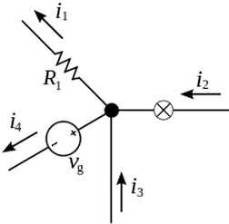
The current entering any junction is equal to the current leaving that junction.

\begin{equation} i_1 + i_4 = i_2 + i_3 \end{equation}

This law is also called Kirchhoff's point rule or Kirchhoff's junction rule (or nodal rule). The more general form the law is stated as The algebraic sum of current at a junction is zero

\begin{equation} \sum_{k=1}^{n}I_k = 0 \end{equation}

Equations 1 and 2 are equivalent as current is a signed (positive or negative) quantity reflecting direction towards or away from a node

Kirchhoff's Voltage Law (KVL)

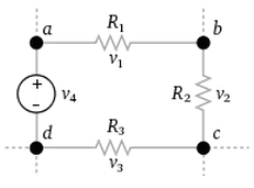
The sum of all the voltages around the loop is equal to zero.

\begin{equation} \sum_{k=1}^{n}V_k = 0 \end{equation}

This law is also called Kirchhoff's second law or Kirchhoff's loop (or mesh) rule. Another way to state this law is The sum of the emf's in a closed circuit is equal to the sum of potential drops

\begin{equation} v_4 = v_1 + v_2 + v_3 \end{equation}

Equations 3 and 4 are equivalent as voltage is a signed (positive or negative) quantity depending whether it is emf and potential drop.

KVL and KCL Examples

Voltage Divider

A voltage divider is a common configuration in analog circuits. It is also known as a potential divider. It is a linear circuit that produces an output voltage (Vout) that is a fraction of its input voltage (Vin). Voltage division refers to the partitioning of a voltage among the components of the divider.

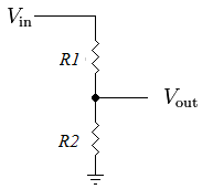
Applying KCL, it can be observed by inspection, that the current i flowing through the resistors R1 and R2 must be equal. Applying KVL \begin{equation} v_{in} = i R_1 + i R_2 \end{equation} \begin{equation} i = {v_{in} \over {R_1 + R_2}} \end{equation} The voltage across R2 is given by \begin{align} v_{out} &= i R_2 \\ \label{vd} &= {R_2 \over {R_1 + R_2}}v_{in} \end{align} This formula is called the voltage divider rule

Loading Effect

The two resistor voltage divider is used often to supply a voltage different from that of an available battery or power supply. In application the output voltage depends upon the resistance of the load (RL) it drives.

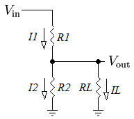
Since RL is parallel to R2 (RL||R2), the output voltage is now given by \begin{equation} v_{out} = {R_2 || R_L \over {R_1 + R_2 || R_L}}v_{in} \end{equation} where \begin{equation} R_2 || R_L = {R_2 R_L \over {R_2 + R_L}} \end{equation}

From KCL, we know that

\begin{equation} I_1 = I_2 + I_L \end{equation}

However if IL (current flowing through RL) can be ignored, then I1 = I2 and the simpler equation \ref{vd} can be used instead. To find the relationship between I2 and IL

\begin{align} V_{out} = I_2 R_2 &= I_L R_L \\ {I_L \over I_2} &= {R_2 \over R_L } \end{align}

In practical circuits, where we can accept resistance tolerance of 10%, IL can be ignored if

\begin{equation} I_L < 0.1 I_2 \end{equation}

Thus we can simplify our analysis by using equation \ref{vd} if

\begin{equation} 10 R_2 < R_L \end{equation}

Input Resistance of BJT Common Emitter Amplifier

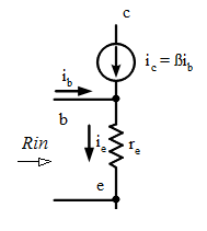
It is a common mistake, without taking into consideration ic, to assume that

\begin{equation} R_{in} = r_e \end{equation}

However when we consider ic, and applying KCL

\begin{equation} i_e = i_b + i_c \end{equation}

Then vre (voltage across re) is

\begin{align} v_{re} &= i_e r_e \\ &= (i_b + \beta i_b) r_e \\ &= (1 + \beta) i_b r_e \end{align}

Assuming β>>1 \begin{align} v_{re} &= \beta i_b r_e \\ R_{in} = {v_{re} \over i_b} &= \beta r_e \end{align}